Covariance matrix
Let \( X \) and \( Y \) be two random variables. The covariance between \( X \) and \( Y \) is defined as:
Let the vector \( Z \) be defined like so: \( Z := \begin{bmatrix} X \\ Y\end{bmatrix} \). Thus, \( Z \) is a vector of random variables.
The covariance matrix for \( Z \) is defined as:
Where the expectation is an elementwise operation. The covariance matrix is a result of a matrix multiplication of two vector-like matrices, which produces a 2x2 matrix. (Yes, it is valid!).
Matrix interpretation
An intepretation of such a 2x1*1x2 matrix multiplication is:
&= \begin{bmatrix}C\begin{pmatrix}A \\ B\end{pmatrix} & D\begin{pmatrix}A \\ B \end{pmatrix} \end{bmatrix}
\end{aligned} \]
The first matrix can be considered a transformation matrix which transforms a single dimension into 2 dimensions. \( A \) is the factor by which the input scalar is multiplied by to produce the first output dimension; \( B \) is the same quantity for the second output dimension. The matrix \( \begin{bmatrix} C & D\end{bmatrix} \) can be considered a list of two separate scalars that will be transformed separately.
For the case of \( Z Z^T \), if \( Z \) has \( D \) dimensions, then the output is D vectors combined horizontally into a matrix, where each vector is the original \( Z \) multiplied by one of it's components.
For the 2 dimensional covariance matrix we have:
Cov[Z] &= E[ (Z - E[Z])(Z - E[Z])^T] \\
&= E\left[ \begin{bmatrix}X - \mu_X \\ Y - \mu_Y \end{bmatrix} \begin{bmatrix}X-\mu_X & Y-\mu_Y\end{bmatrix} \right] \\
&= E[\begin{bmatrix}(X - \mu_X) \begin{pmatrix} X - \mu_X \\ Y - \mu_Y\end{pmatrix} & (Y - \mu_Y) \begin{pmatrix} X - \mu_X \\ Y - \mu_Y\end{pmatrix} \end{bmatrix} ] \\
&= \begin{bmatrix} Cov(X, X) & Cov(Y, X) \\ Cov(X, Y) & Cov(Y, Y) \end{bmatrix} \\
&= \begin{bmatrix} Var(X) & Cov(X, Y) \\ Cov(X, Y) & Var(Y) \end{bmatrix}
\end{aligned} \]
The covariance matrix is symmetric, like all matrixes of the form \( X X^T \). Its diagonal is the variances of each random variable.
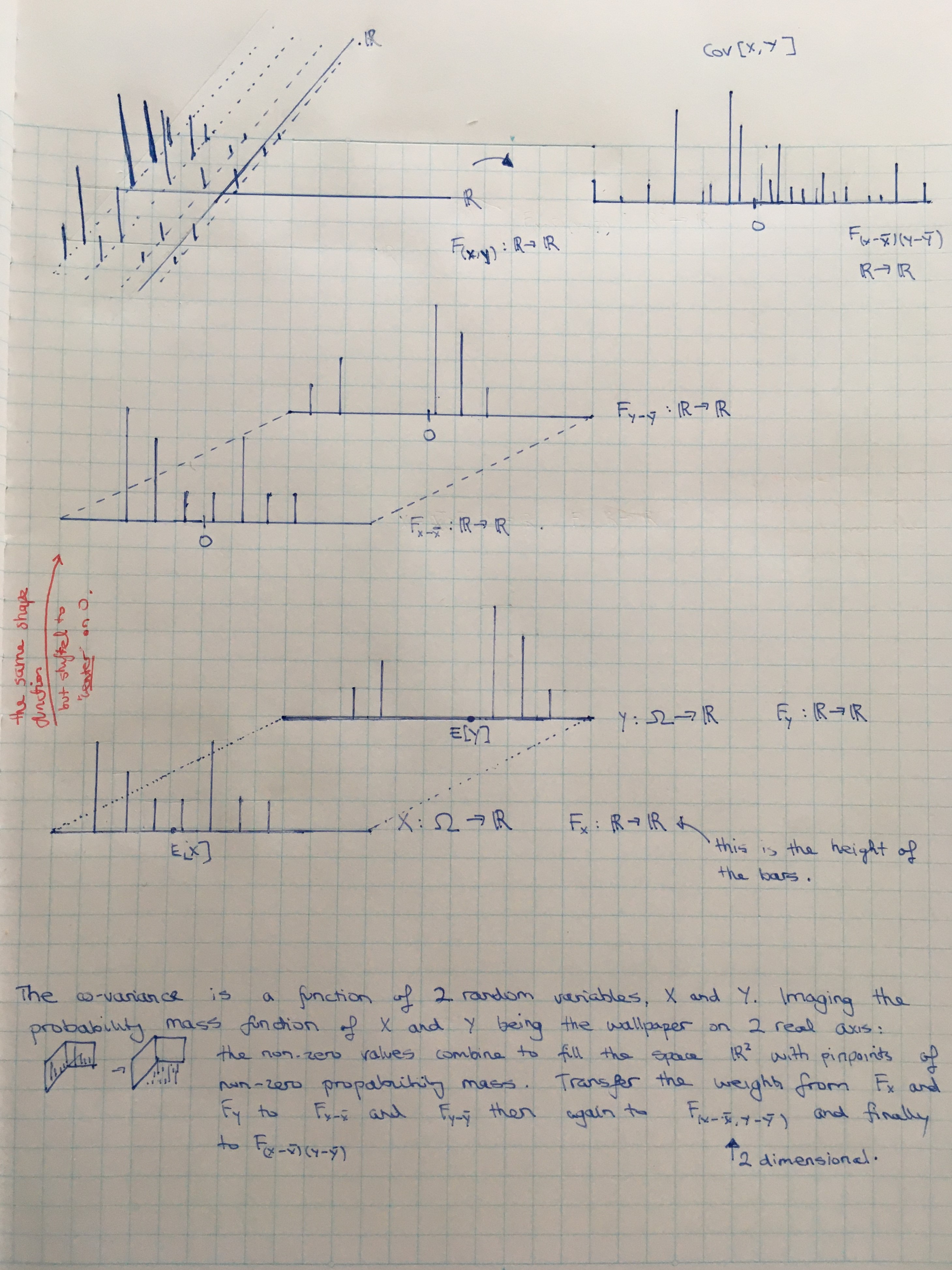
Random variable interpretation
Covariance is the expected value of the random variable \( Z = (X - \bar{X})(Y - \bar{Y}) \). Imagine the probability mass function of \( X \) and \( Y \), then \( X - \bar{X} \) and \( Y - \bar{Y} \), then the 2 dimensional \( (X - \bar{X}, Y- \bar{Y}) \), then finally the 1 dimensional \( Z \). The covariance is a single value representing the expectation (product sum) of the value-probabilities of \( Z \).