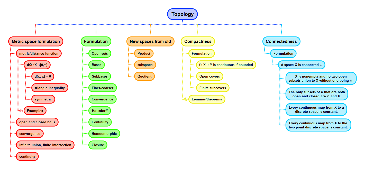
Math and science::Topology
Metric space. ε-balls
Let \( X \) be a metric space, let \( x \in X \) and let \( \varepsilon > 0 \) be a real. The open ε-ball around \( x \) (or in more detail, the open ball around \( x \) of radius \( \varepsilon \)) is the subset of \( X \) given by
\(B(x, \varepsilon) = \{y \in X : d(x, y) < \varepsilon \} \)
Similarly, the closed ε-ball around \( x \) is
\(\bar{B}(x, \varepsilon) = \{y \in X : d(x, y) \le \varepsilon \} \)
The definition of open sets in metric spaces is formulated in terms of open ε-balls.
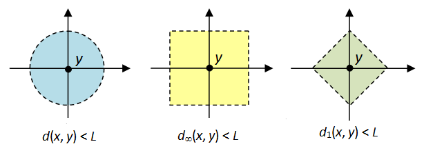
Example
Metrics such as \( d_1 \), \( d_2 \) and \( d_\infty \) for both \( \mathbb{R}^n \) and continuous function spaces \( C[a, b] \), and other metrics such as Hamming distance, each induce ε-balls within the space they are applied in. It is interesting to consider what the ε-ball in each metric space is.
Context